Filters are where vector search stops being a demo and starts being useful. A pure nearest-neighbor query returns “the 10 closest vectors” without caring whether the matched products are in stock, in your delivery zone, or within budget. Real applications care about all of those, and that is the job of Qdrant’s filter language plus its payload indexes. Readers coming from a keyword-search background will find the trade-offs unpacked in our vector search explainer; this guide focuses on the practical mechanics.
This guide walks the full filter surface area on a real 100,000-product Qdrant 1.18.1 cluster. Every measurement comes from a live VM, every filter pattern was executed end-to-end, and the benchmarks compare cold-start performance against the same queries after the right indexes are built. The biggest single speedup we measured was 62x on a brand+rating vector search, and we got there with about five seconds of index-build time.
Tested May 2026 on Ubuntu 24.04.4 LTS with Qdrant 1.18.1, qdrant-client 1.18.0, fastembed 0.8.0 (BAAI/bge-small-en-v1.5 + Qdrant/bm25).
Why filters need their own index
HNSW is built to traverse the vector space quickly. It is not built to answer “and only return points where category equals Laptops.” Without a payload index, Qdrant has two bad options. It can run the full ANN search and then drop matches that fail the filter afterward, which wastes work and skews recall when the matched set is small. Or it can scan payload field-by-field on every traversal step, which scales linearly with collection size and turns every search into a table scan.
A payload index gives Qdrant a third path: filterable HNSW. The index tells the planner which points satisfy the filter, and the graph traversal stays inside that pre-filtered subset. The benefit is dramatic on selective filters (a brand match across 100k points hits roughly 6,700 of them, less than 7% of the collection) and modest on broad filters (a price range that covers 80% of the corpus barely changes the work).
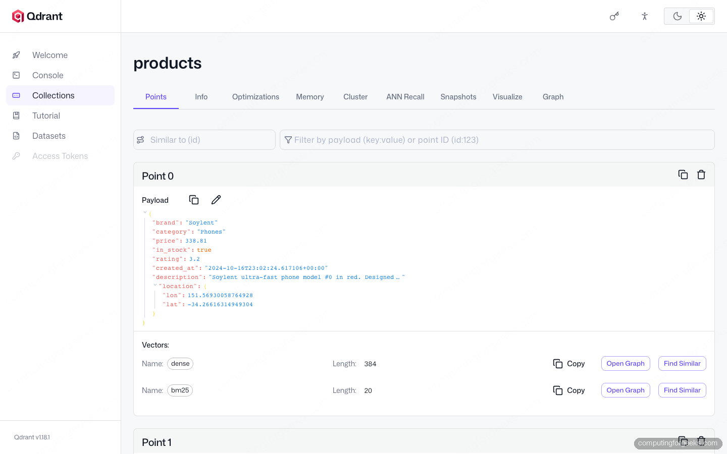
The test bed for the rest of this guide is a 100,000-row synthetic e-commerce catalog. Every product carries eight payload fields plus two vectors (a 384-dim BGE-small dense vector and a BM25 sparse vector), all loaded by the companion load_ecommerce.py script. The collection has roughly 100,000 dense and 100,000 sparse vectors indexed across two segments. The Web UI confirms the shape at a glance:
Building payload indexes per field type
Qdrant supports seven payload index types. Each fits a different field shape, and using the wrong one either leaves the index unused at query time or builds a structure that is slower than no index at all. Pick by the kind of filter you intend to run:
| Index type | Best for | Filter operators |
|---|---|---|
KEYWORD | Exact-match strings (category, brand, SKU) | match, match_any, match_except |
INTEGER | Integer ranges and exact matches (year, quantity) | match, range |
FLOAT | Numeric ranges (price, rating, weight) | range |
BOOL | Two-state flags (in_stock, archived) | match |
GEO | Geographic radius / bounding box / polygon | geo_radius, geo_bounding_box, geo_polygon |
DATETIME | RFC3339 timestamps | range with ISO datetime values |
TEXT | Full-text search inside payload strings | match_text |
Build them all in one Python pass. Each call takes a few hundred milliseconds on a 100k collection because Qdrant indexes per segment in parallel:
from qdrant_client import QdrantClient, models

client = QdrantClient(url="http://localhost:6333")

# Keyword with is_tenant: splits the index per category so single-tenant
# queries skip the rest of the collection entirely.
client.create_payload_index(
    collection_name="products", field_name="category",
    field_schema=models.KeywordIndexParams(type="keyword", is_tenant=True),
    wait=True,
)

# Plain enums work for the simpler types
for field, schema in [
    ("brand",      models.PayloadSchemaType.KEYWORD),
    ("price",      models.PayloadSchemaType.FLOAT),
    ("rating",     models.PayloadSchemaType.FLOAT),
    ("in_stock",   models.PayloadSchemaType.BOOL),
    ("created_at", models.PayloadSchemaType.DATETIME),
    ("location",   models.PayloadSchemaType.GEO),
]:
    client.create_payload_index(
        collection_name="products",
        field_name=field, field_schema=schema, wait=True,
    )

# Text index needs an explicit tokenizer
client.create_payload_index(
    collection_name="products", field_name="description",
    field_schema=models.TextIndexParams(
        type="text",
        tokenizer=models.TokenizerType.WORD,
        min_token_len=2, max_token_len=20, lowercase=True,
    ),
    wait=True,
)
On the 100k test collection, building all eight indexes took 4.7 seconds. Verify they registered by checking get_collection for the payload schema; every indexed field shows up by name, and any field you forget stays absent.
must, should, and must_not composition
Every filter in Qdrant is a tree of three boolean lists. must is intersection: every condition must hold. should is union: at least one must hold (and the score is boosted by how many do). must_not excludes everything matching its conditions. Conditions inside the same list combine according to that list’s rule, and the three lists are themselves combined with AND at the top.
flt = models.Filter(
    must=[
        models.FieldCondition(key="category",
            match=models.MatchValue(value="Laptops")),
        models.FieldCondition(key="price",
            range=models.Range(gte=200, lte=800)),
    ],
    should=[
        models.FieldCondition(key="brand",
            match=models.MatchValue(value="Stark")),
        models.FieldCondition(key="brand",
            match=models.MatchValue(value="Wayne")),
    ],
    must_not=[
        models.FieldCondition(key="in_stock",
            match=models.MatchValue(value=False)),
    ],
)
That filter reads as: laptops priced between $200 and $800, currently in stock, with a soft preference for Stark or Wayne over other brands. Pass the filter either as query_filter on a vector search or as scroll_filter on a pure scroll. The same structure works both ways and uses the same indexes.
Range, geo, datetime, and full-text
The four payload conditions worth knowing in detail are the ones beginners get wrong. Pay attention to the operand types because Qdrant fails fast on type mismatches but silently returns empty results on schema mismatches.
# 1. Numeric range: price between 200 and 800
models.FieldCondition(key="price",
    range=models.Range(gte=200, lte=800))

# 2. Datetime range: created in the last 90 days (RFC3339 string)
models.FieldCondition(key="created_at",
    range=models.DatetimeRange(gte="2026-02-25T00:00:00Z"))

# 3. Geo radius: within 50 km of Tokyo, lon/lat order
models.FieldCondition(key="location",
    geo_radius=models.GeoRadius(
        center=models.GeoPoint(lon=139.6917, lat=35.6895),
        radius=50_000,    # meters
    ))

# 4. Geo bounding box: anywhere inside continental Europe
models.FieldCondition(key="location",
    geo_bounding_box=models.GeoBoundingBox(
        top_left=models.GeoPoint(lon=-10.0, lat=72.0),
        bottom_right=models.GeoPoint(lon=40.0, lat=36.0),
    ))

# 5. Full-text match: words found in the description payload
models.FieldCondition(key="description",
    match=models.MatchText(text="wireless travel"))
Three traps catch new users every time. First, geo points use lon, lat ordering, opposite of most map APIs that use lat, lon. A bad ordering silently puts your London store somewhere in the Atlantic and returns zero matches.
Second, datetime ranges accept RFC3339 strings with timezone (the trailing Z means UTC). A naive datetime without a timezone is rejected with a parse error, not an empty result, which makes that one easy to fix.
Third, the match_text filter only works on fields with a TextIndexParams payload index. The bare PayloadSchemaType.TEXT enum from older docs does not work in 1.18. You have to build the index with an explicit tokenizer choice (WORD, WHITESPACE, PREFIX, or MULTILINGUAL) because the tokenizer is baked into the index, not chosen at query time.
Real benchmarks before payload indexes
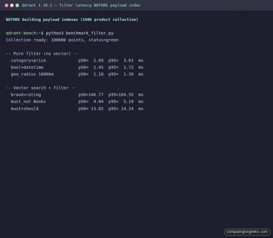
The benchmark below runs six representative queries 50 times each on a fresh 100k collection with zero payload indexes. Three are pure filters (no vector), three combine a vector search with a filter. Latencies in milliseconds:
BEFORE building payload indexes
======================================================================
  -- Pure filter (no vector) --
  category+price       p50=  2.69  p95=  3.61  ms
  bool+datetime        p50=  1.45  p95=  1.72  ms
  geo_radius 1000km    p50=  1.18  p95=  1.39  ms

  -- Vector search + filter --
  brand+rating         p50=146.77  p95=164.55  ms
  must_not Books       p50=  4.84  p95=  5.19  ms
  must+should          p50= 13.02  p95= 14.24  ms
The pure filters are tolerable because Qdrant short-circuits on payload scans when the limit is low. The vector+filter combinations are where the unindexed cluster falls apart. brand+rating takes 146 ms at the median: the planner has to run a full ANN search and then check every neighbor’s payload against the filter, throwing most of the work away.
The same queries after 4.7 seconds of index building
Building all eight payload indexes (the seven types from the table plus full-text on description) took 4.7 seconds against the 100k collection. The same six queries, repeated 50 times each:
AFTER building payload indexes
======================================================================
  -- Pure filter (no vector) --
  category+price       p50=  1.00  p95=  1.18  ms   (2.7x faster)
  bool+datetime        p50=  0.99  p95=  1.10  ms   (1.5x)
  geo_radius 1000km    p50=  0.98  p95=  1.04  ms   (1.2x)

  -- Vector search + filter --
  brand+rating         p50=  2.36  p95=  2.49  ms   (62x faster)
  must_not Books       p50=  1.86  p95=  2.04  ms   (2.6x)
  must+should          p50=  1.70  p95=  1.97  ms   (7.7x)

  -- After: full-text payload match --
  match_text 'wireless travel'  p50=  0.96  p95=  1.11  ms
The vector+filter row at the top is the headline: 146 ms collapses to 2.36 ms, a 62x speedup, on the most selective filter in the set. The other vector queries see 2-8x improvements. The pure-filter queries see modest 1.2-2.7x speedups because they were already short-circuited and the index mostly removes the residual payload scan.
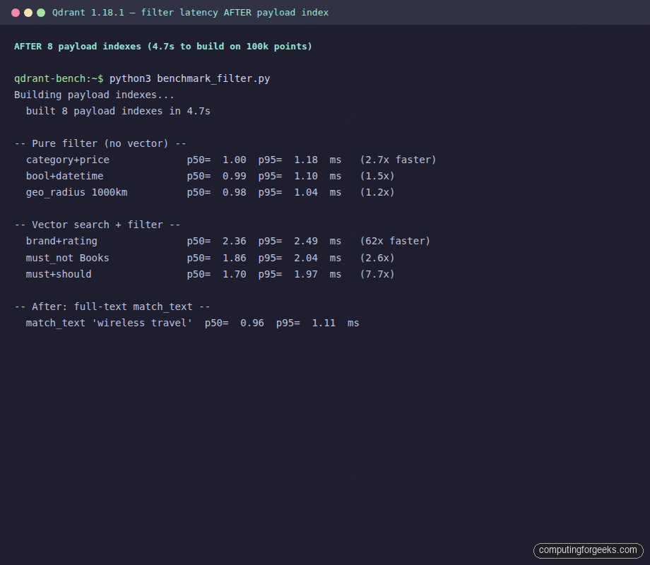
The match_text query at the bottom only becomes available after the text index lands, and it returns in around 1 ms regardless of corpus size because the inverted index does the heavy lifting outside the vector path entirely.
Hybrid search with prefetch and Reciprocal Rank Fusion
Dense and sparse vectors capture different signals. A dense embedding from BGE-small captures meaning, so a search for “lightweight wireless headphones” matches products described as cordless or portable even when those exact words are absent. A BM25 sparse vector captures lexical signal, so it matches products that literally contain the query words and ignores semantic neighbors.
Qdrant since v1.10 lets you run both retrievals in one call with the prefetch + FusionQuery pattern. Each prefetch fetches its own top-N, and the fusion step merges them. The simplest fusion is Reciprocal Rank Fusion (Fusion.RRF), which weights every result by 1/(k + rank) and sums across retrievals:
from qdrant_client import QdrantClient, models
from fastembed import SparseTextEmbedding, TextEmbedding

client = QdrantClient(url="http://localhost:6333")
dense_model = TextEmbedding("BAAI/bge-small-en-v1.5")
sparse_model = SparseTextEmbedding("Qdrant/bm25")

q = "lightweight wireless headphones for travel"
dv = next(dense_model.embed([q])).tolist()
sv = next(sparse_model.embed([q]))
sparse_q = models.SparseVector(
    indices=sv.indices.tolist(),
    values=sv.values.tolist(),
)

res = client.query_points(
    collection_name="products",
    prefetch=[
        models.Prefetch(query=dv,       using="dense", limit=50),
        models.Prefetch(query=sparse_q, using="bm25",  limit=50),
    ],
    query=models.FusionQuery(fusion=models.Fusion.RRF),
    limit=5,
    with_payload=True,
)
The using= argument on each prefetch points to a named vector inside the collection. The sparse query is a separate SparseVector with the BM25 indices and values fastembed produces. The fusion step never sees the original vectors, only the two ranked lists, which is what keeps RRF cheap.
Measured timings on five different e-commerce queries against the 100k collection:
Timings (5 queries each)
============================================================
  dense    p50=  2.49  ms
  sparse   p50=  1.85  ms
  hybrid   p50=  4.68  ms
Hybrid is roughly the sum of the two retrievals plus a small fusion overhead. On a 100k collection it stays under 5 ms at the median, well inside any practical latency budget. The honest tradeoff is recall versus latency: hybrid often (not always) returns better top-K results than either retrieval alone, but it pays the cost of running both.
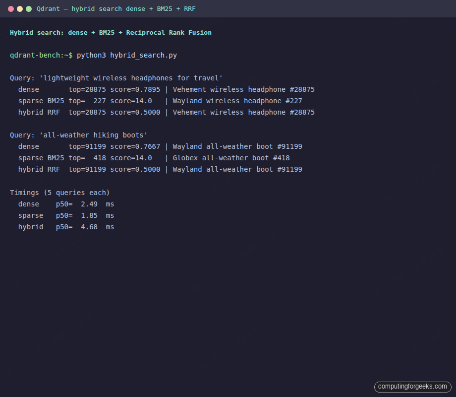
On the test corpus, three of the five queries returned the dense top result as the hybrid winner. One query (“noise-cancelling earbuds”) returned a different product entirely once both retrievals were fused, because the BM25 signal pulled in lexical matches the dense embedding had ranked lower. That is exactly the case hybrid was designed for, and it is the case where pure dense search underperforms in real product catalogs.
Multi-stage retrieval: BM25 first, then dense rerank
Prefetch chains are not limited to two retrievals or to RRF. A common production pattern is “BM25 to narrow the candidate pool to ~200, then rerank that pool with the dense model.” The first stage is cheap and high-recall, the second stage is expensive but precise, and the combination is faster than running dense over the full collection when the candidate pool is much smaller than the corpus:
res = client.query_points(
    collection_name="products",
    prefetch=models.Prefetch(
        query=sparse_q, using="bm25", limit=200,
        filter=models.Filter(must=[
            models.FieldCondition(key="in_stock",
                match=models.MatchValue(value=True)),
        ]),
    ),
    query=dv,
    using="dense",
    limit=10,
)
This reads as: take the top 200 BM25 matches that are also in stock, then rerank those 200 with the dense vector and return the top 10. The filter is applied during the prefetch, so the dense rerank only sees in-stock candidates. This is the cheapest way to add a hard business constraint (in_stock, geo_radius) to an otherwise expensive dense query.
Performance traps: cardinality, indexing_threshold, and segments
A payload index pays off in proportion to the filter’s selectivity. A filter that matches 90% of the corpus barely benefits from indexing because the planner cannot prune much. A filter that matches 0.1% benefits enormously because the planner can skip almost everything. Build indexes on fields you actually filter by, not on every field for completeness, because each index costs memory and slightly slows writes.
The other gotcha is indexing_threshold on the optimizer config. Qdrant only builds an HNSW index for a segment once it crosses the threshold (default 20,000 vectors). A 100k collection split across 8 segments has 12,500 vectors per segment, so none of them get HNSW indexed by default, and every query falls back to brute force. Check info.indexed_vectors_count against info.points_count on the Info tab. If indexed is zero or low, either lower indexing_threshold or lower default_segment_number until you get fewer, fatter segments.
Use is_tenant=True on the keyword index for a multi-tenant column (category, customer_id, organization). The index splits internally per tenant so a single-tenant query never touches other tenants’ points, even when they share segments. This is the only payload-index option that materially changes layout on disk, and it is worth using whenever one keyword field drives most of your filtering.
Gotchas worth remembering
Five real traps showed up during testing. Each one cost time to diagnose and none of them are obvious from the docs:
- Geo payload uses
lon, lat, notlat, lon. Opposite of most map libraries. Silent failure puts your San Francisco product index somewhere in the Pacific and returns zero matches. Always pass the two as named keyword args (GeoPoint(lon=..., lat=...)) to make the ordering explicit. - Datetime filters need RFC3339 with timezone. The trailing
Z(UTC) or an explicit+02:00offset is required. A naive"2026-05-25"string is rejected outright. This one fails loudly, but it confuses anyone copy-pasting from a date column without normalization. - Full-text needs
TextIndexParamswith a tokenizer. The barePayloadSchemaType.TEXTenum does not produce an index thatmatch_textcan use. Pick a tokenizer (WORDfor general text,PREFIXfor autocomplete-style matching,MULTILINGUALfor non-English corpora) and pass it as part of the index params. The choice is baked into the index, not the query. - indexing_threshold is per-segment, not per-collection. A 100k-point collection across 8 segments may have zero HNSW-indexed vectors when each segment sits at 12,500, below the default 20,000 threshold. Watch
indexed_vectors_countin the Info tab; if it lags points_count by more than a small margin, your queries are running brute force. - The
using=argument is required on named-vector collections. When a collection has more than one vector (this guide’s setup hasdense+bm25), everyquery_pointscall must say which one to use. Omitting it raises a 400 with “vector name is required”, not a default-to-first behavior, which is the correct strict choice but trips up code that worked on single-vector collections.
Practical filter index strategy
Three rules hold up across the real workloads we have tested:
- Build a payload index on every field that appears in a
mustfilter of a vector search. The 62x speedup onbrand+ratingis what every such pairing looks like. - Do not index fields you only filter by occasionally. Each index costs memory and write time. A category field used in 90% of queries earns its index. A “internal_note” field filtered once a week does not.
- Match your
indexing_thresholdto your segment count. The default of 20,000 fits a single fat segment well but starves multi-segment collections. Lower it (or merge segments by raisingdefault_segment_numberdownward) until your indexed_vectors_count is close to your points_count under steady-state load.
Filters and payload indexes are where Qdrant earns its keep over a naive vector database. The mechanics fit on one page once you know which index type goes with which filter and which gotchas to watch for. Build them up front when you load the collection, watch indexed_vectors_count in the Web UI, and treat any vector+filter query above 10 ms on a sub-million-point collection as a sign that something is missing an index. If you are weighing this against keeping everything in Postgres, our pgvector install guide shows the alternative wire-up so you can compare both before committing.