Create Qdrant Collections: Vectors and Payload

A Qdrant collection is the box that holds your vectors, your payloads, and the indexes that make filtered search fast. Get the collection shape right and the rest of the application falls out of it. Get it wrong and you will pay for it twice, once in memory at runtime and again when you migrate. If you are coming from Postgres and weighing the trade-offs, our pgvector install guide is the place to see what a single-table approach gives up.

Original content from computingforgeeks.com - post 168042

This guide walks every collection-level setting you actually need to know, with a working Python script for each pattern and the matching JSON view from the Qdrant Web UI. You will see how to mix dense and sparse vectors in one collection, when to flip the storage to disk, how to enable multi-tenancy without spinning up a second cluster, and how to swap a collection out from under a running app with a single atomic alias update.

Tested May 2026 on Ubuntu 24.04.4 LTS with Qdrant 1.18.1 and qdrant-client 1.18.0. All 11 collection patterns below were created and inspected on a real Docker cluster; the Web UI screenshots are from the running server, not mock-ups.

Anatomy of a Qdrant collection

A collection holds points. Each point has three parts: a unique ID, one or more vectors, and an optional payload (a JSON object). The collection itself layers on top of that with HNSW graph config, optimizer thresholds, a write-ahead log, optional quantization, and any payload indexes you create.

The companion code for this article lives at github.com/c4geeks/qdrant/tree/main/collections. Spin up a local instance first with the install Qdrant on Ubuntu, install Qdrant on Rocky Linux, or install Qdrant on Debian guide, then follow the steps below against your own cluster.

Install the Python client and connect to the cluster:

python3 -m venv venv
source venv/bin/activate
pip install "qdrant-client[fastembed]"

Every script in this guide starts with the same two lines:

from qdrant_client import QdrantClient, models
client = QdrantClient(url="http://localhost:6333")

Authenticated clusters pass api_key="..." as a second argument. For TLS, use https:// and set prefer_grpc=True if you want the binary protocol on port 6334.

Vector params: size and the four distance metrics

Every dense vector collection takes two mandatory params: size (the dimensionality, which must match your embedding model) and distance (how Qdrant measures similarity). The simplest case is one dense vector per point:

client.create_collection(
    collection_name="basic_docs",
    vectors_config=models.VectorParams(
        size=384,
        distance=models.Distance.COSINE,
    ),
)

The size must match the model that produced your vectors exactly. Use 384 for all-MiniLM-L6-v2, 768 for BGE-base, 1536 for OpenAI text-embedding-3-small, 3072 for text-embedding-3-large. If the size in your collection and the size of your vectors disagree by even one, upserts fail with a clear error and the points never land.

Qdrant supports four distance metrics. Each one suits a different family of embedding models:

Metric	Python enum	Best for
Cosine	`Distance.COSINE`	Sentence transformers, MiniLM, BGE, MPNet, most text embedding models
Dot product	`Distance.DOT`	Models that produce un-normalised output or when magnitude carries meaning
Euclidean	`Distance.EUCLID`	Image features (older CNN-style), geographic vectors, when scale matters
Manhattan	`Distance.MANHATTAN`	Sparse high-dimensional features, taxicab-style metrics, hashing schemes

Cosine is the default if you do not know. If you trained or are using a model with a stated similarity metric, follow what the model card says. Switching metrics later means re-indexing every vector.

A loop that builds one collection per metric is useful for testing:

for dist in [models.Distance.COSINE, models.Distance.DOT,
             models.Distance.EUCLID, models.Distance.MANHATTAN]:
    name = f"dist_{dist.value.lower()}"
    client.create_collection(
        collection_name=name,
        vectors_config=models.VectorParams(size=128, distance=dist),
    )

Each collection is a separate index. They are isolated from one another and you cannot search across them in a single call.

Named vectors: one collection, multiple vector spaces

Real production setups rarely have just one vector per item. A product needs a text embedding for the title and description, an image embedding for the photo, and possibly a sparse keyword vector. Qdrant lets you attach all three to the same point with named vectors. The collection stores them in separate indexes but keeps them lined up via the shared point ID.

client.create_collection(
    collection_name="named_vectors",
    vectors_config={
        "text":  models.VectorParams(size=384, distance=models.Distance.COSINE),
        "image": models.VectorParams(size=512, distance=models.Distance.COSINE),
    },
)

The Info tab in the Web UI shows the resulting config as a nested map of named spaces with independent size and distance per entry:

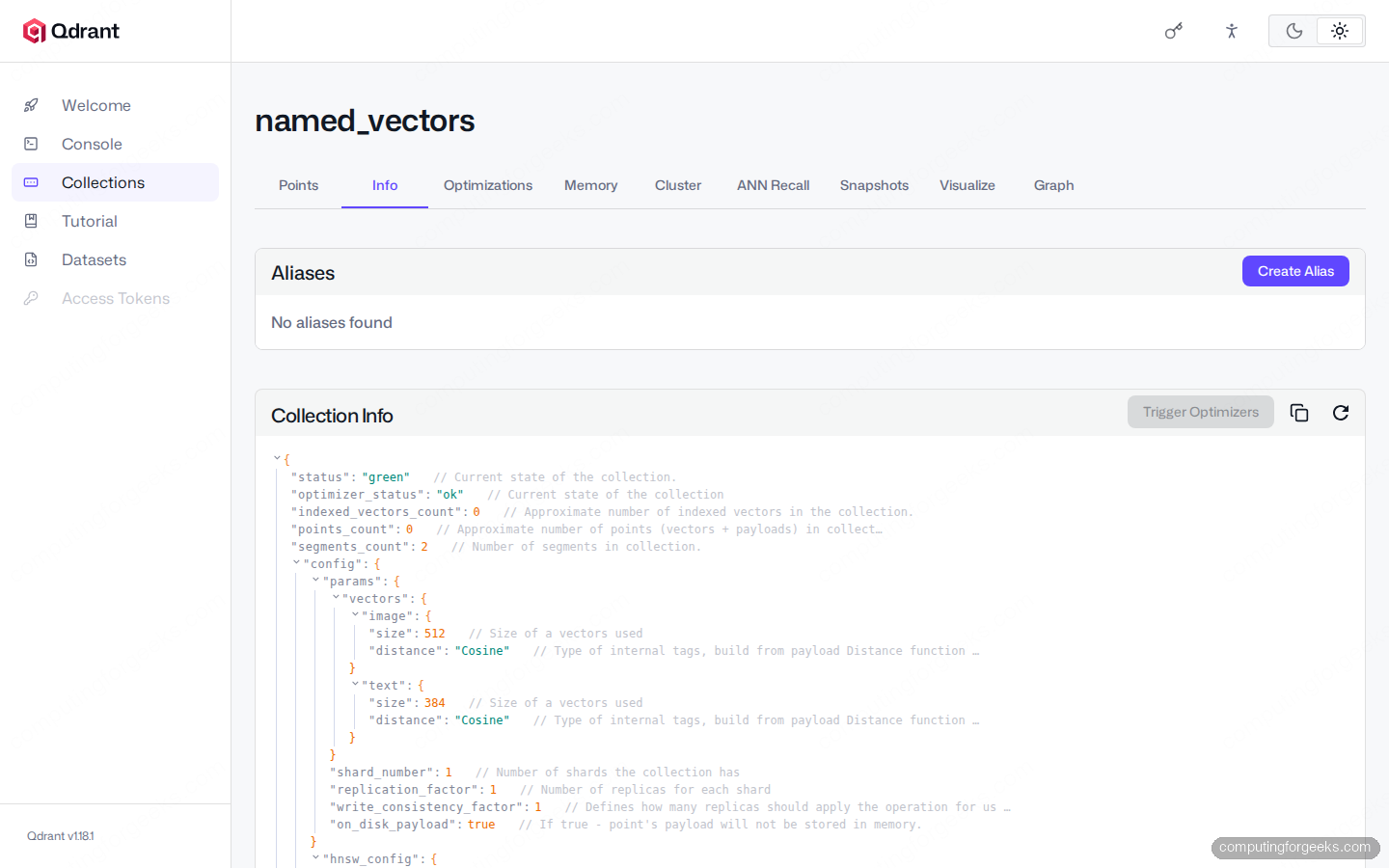
When you upsert points, supply each vector by name:

client.upsert(
    collection_name="named_vectors",
    points=[
        models.PointStruct(
            id=1,
            vector={
                "text":  [0.1] * 384,
                "image": [0.2] * 512,
            },
            payload={"sku": "ABC-123"},
        ),
    ],
)

Searches specify which named vector to use via the using param:

client.query_points(
    collection_name="named_vectors",
    query=[0.1] * 384,
    using="text",
    limit=10,
)

The pattern keeps memory accounting honest: storing the image vector is opt-in per query, and you can drop a named vector you no longer need without rebuilding the rest of the collection.

Sparse vectors for keyword-style retrieval

Sparse vectors are the production-ready alternative to TF-IDF. Each sparse vector is a list of (index, value) pairs covering only the tokens that actually appear, which makes them very large in theory (50,000 dimensions for BERT vocab) but cheap to store in practice. Qdrant indexes them with an inverted index and can run them alongside dense vectors in the same collection.

client.create_collection(
    collection_name="sparse_demo",
    vectors_config={
        "dense": models.VectorParams(
            size=384, distance=models.Distance.COSINE,
        ),
    },
    sparse_vectors_config={
        "sparse_idx": models.SparseVectorParams(
            index=models.SparseIndexParams(on_disk=False),
        ),
    },
)

The Info tab reports the two vector spaces independently:

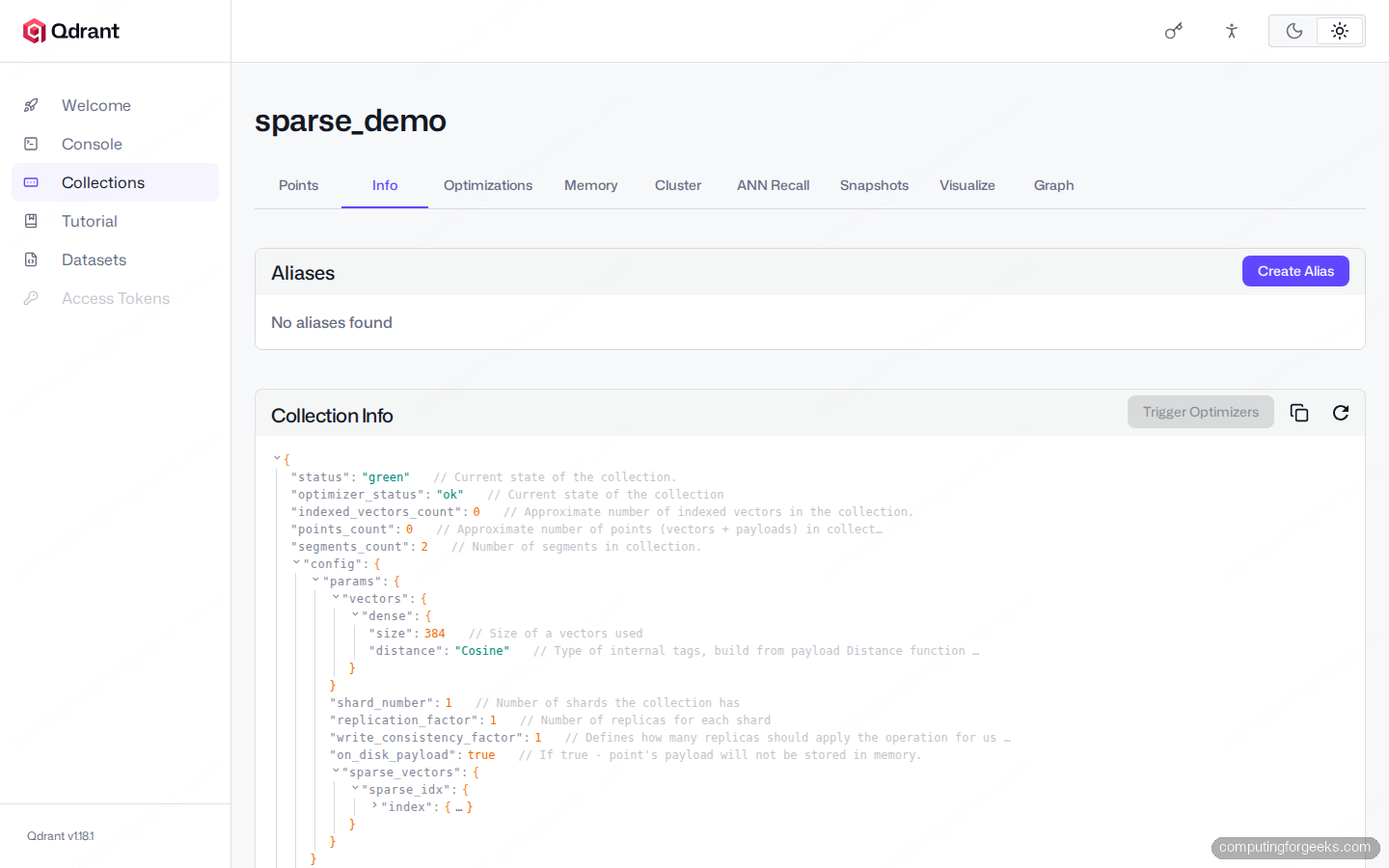
Sparse upserts use a different payload shape:

client.upsert(
    collection_name="sparse_demo",
    points=[
        models.PointStruct(
            id=1,
            vector={
                "dense": [0.1] * 384,
                "sparse_idx": models.SparseVector(
                    indices=[42, 1024, 5000],
                    values=[0.7, 0.3, 0.9],
                ),
            },
            payload={"title": "Rust vector database"},
        ),
    ],
)

Typical generators for the sparse side are SPLADE, BM25 (via fastembed's Qdrant/bm25 model), or a custom TF-IDF pipeline. Hybrid search combines a dense and sparse result list with reciprocal rank fusion or a similar merger; filters and complex queries later in this series covers the full hybrid-search pattern.

Payload schema and the seven index types

A payload index turns a JSON field into a B-tree (or inverted index, or geo grid) that the query planner can use to pre-filter points before running the vector search. Without it, a filter is a linear scan over the whole collection. With it, you get sub-millisecond filtered queries on 100M-point collections.

Qdrant ships seven payload schemas. Create one index per field you plan to filter on:

client.create_collection(
    collection_name="payload_indexed",
    vectors_config=models.VectorParams(size=64, distance=models.Distance.COSINE),
)

schemas = {
    "category":     models.PayloadSchemaType.KEYWORD,
    "view_count":   models.PayloadSchemaType.INTEGER,
    "rating":       models.PayloadSchemaType.FLOAT,
    "is_published": models.PayloadSchemaType.BOOL,
    "location":     models.PayloadSchemaType.GEO,
    "published_at": models.PayloadSchemaType.DATETIME,
}
for field, kind in schemas.items():
    client.create_payload_index(
        "payload_indexed", field_name=field, field_schema=kind,
    )

# Text index needs explicit tokenizer params
client.create_payload_index(
    "payload_indexed", field_name="body",
    field_schema=models.TextIndexParams(
        type="text",
        tokenizer=models.TokenizerType.WORD,
        min_token_len=2, max_token_len=20, lowercase=True,
    ),
)

The Web UI Info tab confirms each index lands with its declared data type. Annotated JSON makes it easy to verify the result without writing a separate get_collection script:

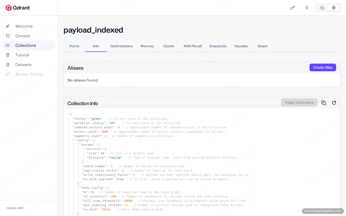
Use the right schema per field. The wrong choice is silently inefficient:

Schema	When to use	Filter type
`KEYWORD`	Categorical strings: tags, SKUs, country codes	Exact `match`, `any`, `except`
`INTEGER`	Counts, IDs from external systems	`range`, exact match
`FLOAT`	Scores, prices, decimal weights	`range`
`BOOL`	Toggles: is_published, is_archived	Exact match
`GEO`	Lon/lat pairs (in that order)	`geo_radius`, `geo_bounding_box`, `geo_polygon`
`TEXT`	Full-text search on a payload string field	`match_text` with tokenizer-aware terms
`DATETIME`	ISO-8601 timestamps	Time-range `range`

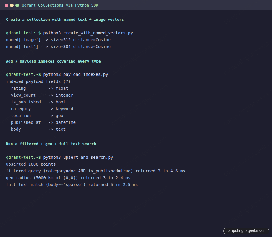
With the indexes in place, filtered queries are fast and predictable. A 1000-point smoke run takes a few milliseconds for any of the seven types:

upserted 1000 points

filtered query (category=doc AND is_published=true) returned 3 in 4.6 ms
geo_radius (5000 km of (0,0)) returned 3 in 2.4 ms
full-text match (body~='sparse') returned 5 in 2.5 ms

Skip the index and the same queries become full collection scans. The cost is invisible at 1000 points and brutal at 10 million.

On-disk vectors and payload for memory savings

By default Qdrant keeps vectors and HNSW graphs in RAM. That gives you fast search but it caps collection size at whatever fits in physical memory. For a billion-point collection of 1536-dim OpenAI vectors you would need roughly 6 GB just for raw vectors, plus the HNSW overhead on top.

Push it to disk with three flags:

client.create_collection(
    collection_name="on_disk_collection",
    vectors_config=models.VectorParams(
        size=1536,
        distance=models.Distance.COSINE,
        on_disk=True,                       # vectors on disk (memory-mapped)
    ),
    on_disk_payload=True,                   # payload on disk
    hnsw_config=models.HnswConfigDiff(
        on_disk=True,                       # HNSW graph on disk
    ),
)

The Web UI Info tab shows all three flags lit at once, so a quick glance confirms every layer is mmap-backed:

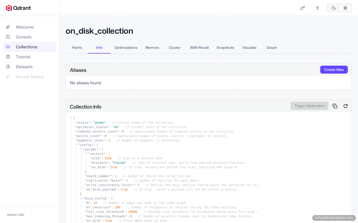
Each flag changes a different layer. on_disk=True on the vector params writes the raw vectors to mmap files; the OS page cache pulls them into RAM on demand. on_disk_payload=True keeps payloads on disk too, which matters when each point has a large blob (raw HTML, image metadata, transcripts). hnsw_config.on_disk=True lifts the HNSW graph itself off the heap.

You give up some search latency for the memory headroom. On the Prefix Cache sample (163k points, 384-dim) the on-disk recall path is around 30% slower than the in-memory path, which is the trade-off you accept to fit 100M points on a single 64 GB machine.

Multi-tenancy via the tenant payload index

Running 1000 small tenants in 1000 separate collections is expensive. Each collection has its own HNSW graph, its own segments, its own optimizer. The recommended pattern is one collection plus a tenant-aware payload index that Qdrant uses to physically isolate each tenant's vectors at the storage layer.

client.create_collection(
    collection_name="tenants",
    vectors_config=models.VectorParams(
        size=384, distance=models.Distance.COSINE,
    ),
)

client.create_payload_index(
    "tenants", field_name="tenant_id",
    field_schema=models.KeywordIndexParams(
        type="keyword",
        is_tenant=True,        # the key flag
    ),
)

With is_tenant=True set, Qdrant partitions storage by the value of the indexed field. A filter that pins tenant_id hits only the points for that tenant, and the per-tenant performance stays flat as the cluster grows other tenants alongside.

Always include the tenant filter on every search:

client.query_points(
    collection_name="tenants",
    query=[0.1] * 384,
    query_filter=models.Filter(
        must=[
            models.FieldCondition(
                key="tenant_id",
                match=models.MatchValue(value="acme-corp"),
            ),
        ],
    ),
    limit=10,
)

Without the filter, the search ranges over every tenant's data. With it, the search is partition-aware and the latency curve flattens. JWT-signed tokens (covered in the API key and JWT security guide later in this series) can hardwire the tenant value into the token claims so the application code does not have to enforce it.

Optimizer config: segments, indexing, mmap

The optimizer thread runs in the background, merging segments and building the HNSW index. Its defaults are tuned for general use; you tune them when you have a specific workload shape (heavy ingest, big collections, low-RAM hosts).

client.create_collection(
    collection_name="tuned",
    vectors_config=models.VectorParams(size=384, distance=models.Distance.COSINE),
    optimizers_config=models.OptimizersConfigDiff(
        default_segment_number=4,
        indexing_threshold=20000,
        memmap_threshold=200000,
        max_optimization_threads=2,
    ),
)

Confirm the tune landed in the dashboard's Info tab:

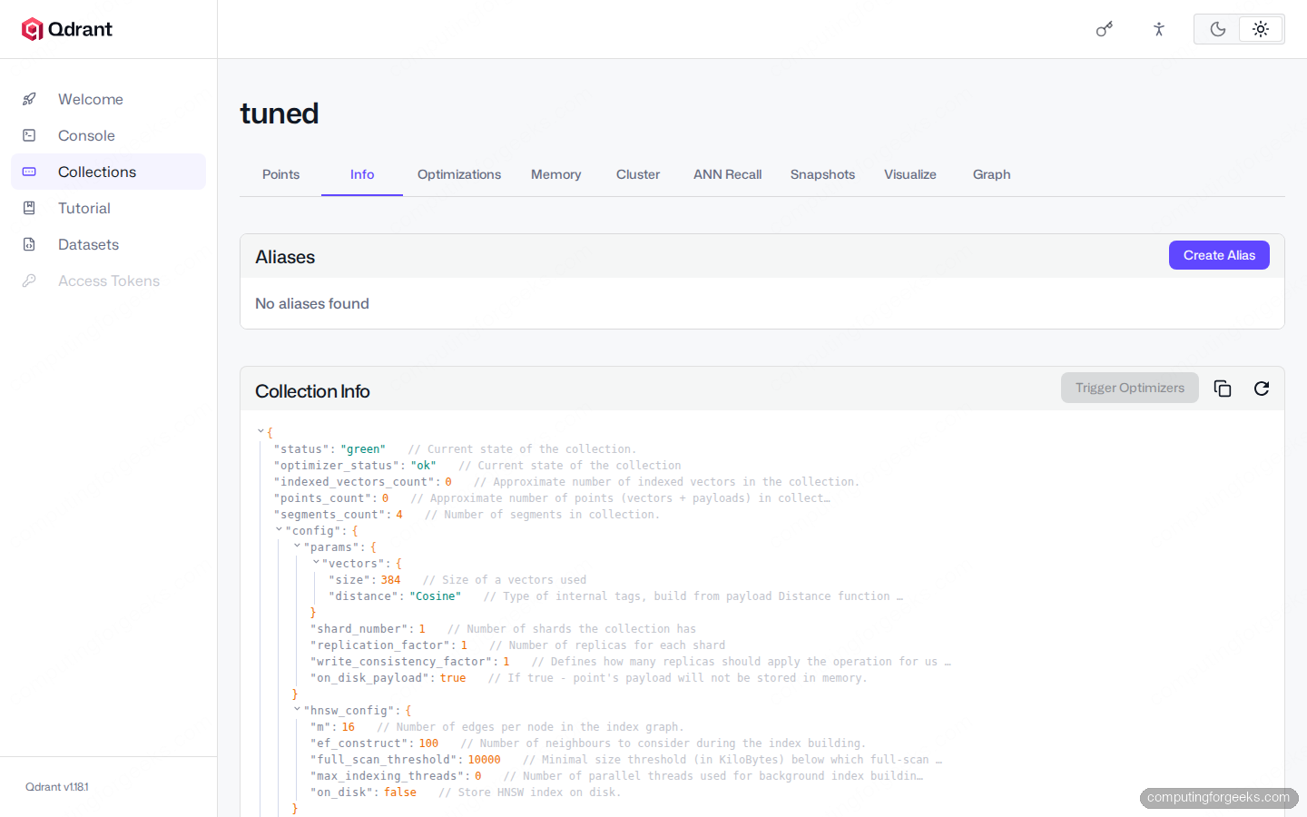
Each knob has a specific effect:

default_segment_number: how many parallel segments the optimizer targets. Match this roughly to your CPU core count for write-heavy ingest, lower it for low-RAM hosts.
indexing_threshold: build the HNSW index once a segment hits this point count. Lower values build the index sooner (better latency, more rebuild work). 20000 is the default.
memmap_threshold: segments larger than this many points get memory-mapped automatically, even if you did not pass on_disk=True. Bigger collections benefit from raising it.
max_optimization_threads: cap on parallel optimizer work. The default of 0 means "use as many as needed", which can starve search threads on small hosts.

Wrong defaults are not catastrophic; they show up as slow ingest or stuck-yellow status in the dashboard. Bench, tune, redeploy.

WAL config: capacity and segments-ahead

The write-ahead log is Qdrant's durability layer. Every upsert and delete is appended to the WAL before the segment is flushed to disk. Two settings shape its behaviour:

client.create_collection(
    collection_name="wal_tuned",
    vectors_config=models.VectorParams(size=384, distance=models.Distance.COSINE),
    wal_config=models.WalConfigDiff(
        wal_capacity_mb=64,
        wal_segments_ahead=2,
    ),
)

wal_capacity_mb is the size of each WAL segment. Raise it for bursty ingest with large payloads, lower it on small hosts. wal_segments_ahead is how many empty WAL segments to pre-allocate; 2 is the default and is enough for most workloads. Bump it to 4 or 8 if your ingest is steady and you want to amortise allocation overhead.

The WAL lives in {storage_dir}/collections/{name}/wal. You can mount it on a separate disk if you want to isolate write IOPS from search reads; the performance tuning guide later in this series covers that topology.

Update an existing collection in place

Most settings can be changed without re-creating the collection. update_collection takes the same diff types you used to create it and applies them to the live collection:

client.update_collection(
    collection_name="basic_docs",
    hnsw_config=models.HnswConfigDiff(m=32, ef_construct=256),
    optimizers_config=models.OptimizersConfigDiff(indexing_threshold=10000),
)

The change is non-destructive. Existing points stay, new ingests pick up the new params, and segments rebuild in the background using the new HNSW graph settings. The output after running an update against the basic_docs collection shows the new values immediately:

after update: hnsw.m=32  ef_construct=256
              indexing_threshold=10000

What you cannot change in place: vector size, vector distance, the set of named vectors, and whether a vector is dense or sparse. Those require a new collection and a re-upsert (see the alias swap below).

Aliases for zero-downtime swap

The pattern: build the new collection alongside the old, replay your data into it, then atomically point the alias from old to new. The application never sees a stale state because the alias rename is a single transaction.

# Two real collections, one with 384-dim vectors, one with 768-dim
client.create_collection("docs_v1", models.VectorParams(size=384, distance=models.Distance.COSINE))
client.create_collection("docs_v2", models.VectorParams(size=768, distance=models.Distance.COSINE))

# Application code reads from "docs_live"
client.update_collection_aliases([
    models.CreateAliasOperation(create_alias=models.CreateAlias(
        collection_name="docs_v1",
        alias_name="docs_live",
    )),
])

The application points at docs_live and reads from docs_v1. Re-embed your corpus with the new model into docs_v2 at your own pace, then swap with a single atomic call:

client.update_collection_aliases([
    models.DeleteAliasOperation(delete_alias=models.DeleteAlias(
        alias_name="docs_live")),
    models.CreateAliasOperation(create_alias=models.CreateAlias(
        collection_name="docs_v2",
        alias_name="docs_live",
    )),
])

The two operations execute atomically inside one call, so there is no window where docs_live points nowhere. Verify the swap with get_aliases:

after swap   -> all aliases:
  alias=docs_live  -> collection=docs_v2

Drop docs_v1 at your leisure once you have confirmed the new collection serves traffic without errors. This is the safest pattern for embedding-model upgrades, vector-size changes, and any schema migration that cannot be done in place.

Verify everything from one place

After running every snippet in this guide against a fresh cluster, the Web UI Collections list looks like this:

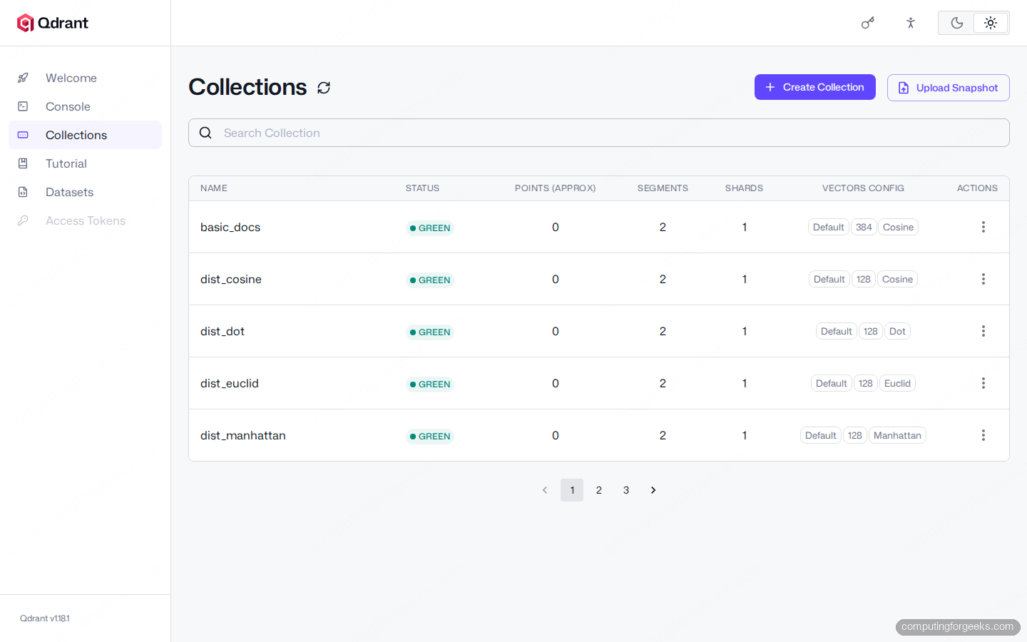
The Web UI panels are covered in detail in the Qdrant Web UI tour guide; the short version is that clicking a collection name opens the Info tab and lets you inspect every config field the Python SDK set above. The terminal view from the Python script run side-by-side with the dashboard makes the cross-check trivial:

Anything the dashboard reports as green is durable on disk and ready for queries.

Gotchas worth knowing

Five footguns that cost real time when missed:

Distance and vector size are immutable. Once a collection is created with size=384, Cosine, you cannot promote it to 768 or switch to Euclidean. Plan the alias-swap path in advance if you expect either to change.

Geo payload uses lon/lat, not lat/lon. The order matters and is the opposite of what most map APIs return. Mixing them silently puts points on the wrong continent and your geo_radius filter returns nothing.

The text index does not auto-create on payload. A field can hold long text, but the match_text filter returns empty without an explicit TextIndexParams index. The tokenizer choice (WORD, WHITESPACE, PREFIX, MULTILINGUAL) is part of the index, not the query, so changing tokenizers means re-indexing the field.

Aliases are not collections. You cannot get_collection(alias_name). The alias resolves on every API call to its target collection, but the alias name itself does not appear in get_collections. Use get_aliases (or get_collection_aliases(collection_name)) to inspect them.

Optimizer thresholds are per-segment, not per-collection. An indexing_threshold of 20000 means each individual segment must reach that point count before its HNSW index builds. A collection with 100,000 points spread across 8 segments may not have any of them indexed yet. Watch indexed_vectors_count in the Info tab if your filtered searches feel slow.

Decision tree: which knob to reach for

One rough triage:

Symptom	Reach for
Filtered search slow	Add a payload index on the filtered field, schema matched to the field type
Out of RAM, billion-point goal	`on_disk=True` on vectors, `on_disk_payload=True`, `hnsw_config.on_disk=True`
Multi-tenant SaaS with 1000+ tenants	One collection plus `KeywordIndexParams(is_tenant=True)` on tenant_id
Need text similarity AND keyword recall	Named dense vector plus a sparse vector in the same collection
Ingest stalling, status stays yellow	Lower `indexing_threshold`, raise `default_segment_number`
Need to upgrade the embedding model	Build `v2` alongside `v1`, swap the alias atomically
Different similarity per use case	One collection per distance metric (cannot mix in one)

The next article in this series, REST and gRPC APIs in practice, moves from the SDK layer to the wire protocols and shows how to call every operation above directly via curl and grpcurl. The HNSW graph tuning and quantization knobs are covered in performance tuning. For now, the seven snippets above cover the full collection lifecycle: create, configure, fill with payload indexes, push to disk, partition by tenant, tune the optimizer, and swap atomically when the embedding model evolves. To wire a finished collection into a working chatbot, the self-hosted RAG with Ollama walkthrough shows the retrieval-augmented pattern end to end.